Simulation
Peter Alping
May 24, 2018
- Introduction
- Basics
- Linear Regression
- Logistic Regression
- Confounding
- Selection Bias
- Generalized Linear Models
Introduction
Simulation is the imitation of the operation of a real-world process or system – Wikipedia
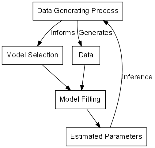
Our typical situation
We want to know more about a biological process for which we have measured data
- An biological process generates data
- We measure and collect this data
- Invent model how we think data was generated
- Fit the model to our data
- Giving us the parameters for the model
- Inferences about the data-generating process
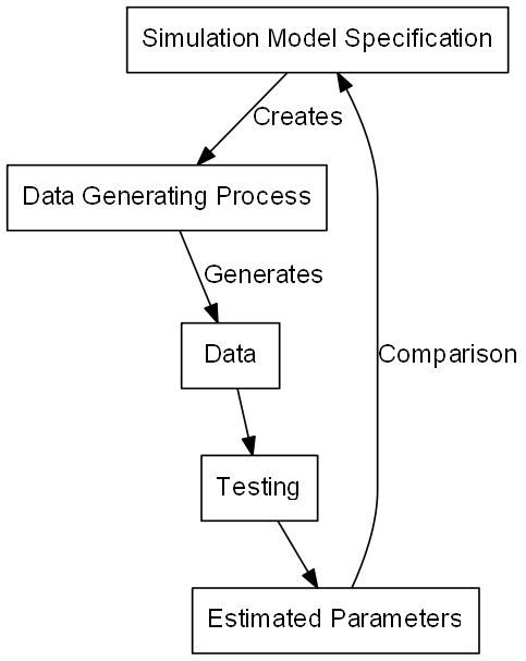
The simulation situation
We want to know more about how something behaves, given data of specific type
- Specify a model for the simulated data
- Including model parameters
- Generate data using this model
- Test something given our data
- Compare the result to our “true” model
Basics
Linear Regression
When do we use it?
- Continuous dependent variable (y)
- Cont./discrete independent variables (x_1, ..., x_p)
- Error normally distributed
- y = \beta_0 + \beta_1x_1 + \beta_2x_2 + ... + \beta_px_p + \epsilon
- \epsilon \sim normal(0, \sigma)
In GLM notation
- Dependent variable from normal distribution (y)
- Cont./discrete independent variables (x_1, ..., x_p)
- E(y) = \mu = \beta_0 + \beta_1x_1 + \beta_2x_2 + ... + \beta_px_p
- y \sim normal(\mu, \sigma)
Logistic Regression
When do we use it?
- Binary dependent variable (y)
- Cont./discrete independent variables (x_1, ..., x_p)
- No common error distribution independent of predictor values
- logit(y) = \beta_0 + \beta_1x_1 + \beta_2x_2 + ... + \beta_px_p + \epsilon
- logit(y) = log(\frac{y}{1 - y})
- \epsilon has no independent distribution
In GLM notation
- Dep. var. from binomial distr. with 1 trial (y)
- Cont./discrete independent variables (x_1, ..., x_p)
- E(y) = \mu = logit^{-1}(\beta_0 + \beta_1x_1 + \beta_2x_2 + ... + \beta_px_p)
- logit^{-1}(x) = \frac{e^x}{1 + e^x}
- y \sim binomial(1, \mu)
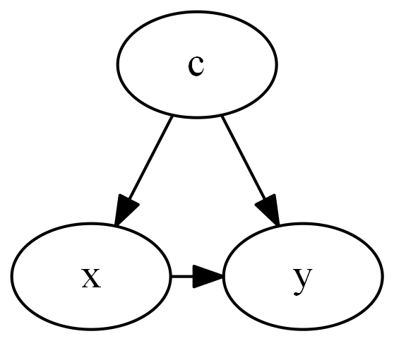
Confounding
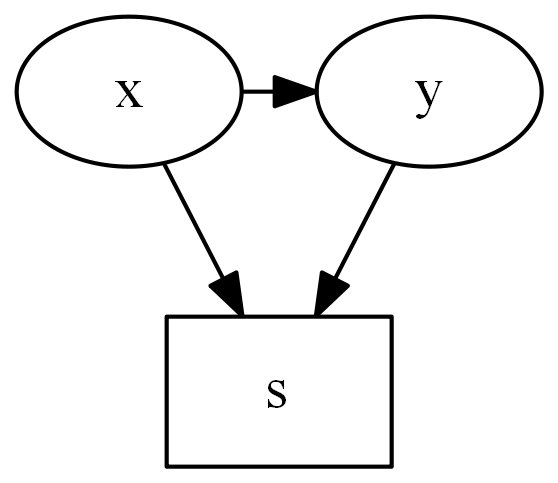
Collider Stratification Bias
Generalized Linear Models
Generalized Linear Models
- E(y) = \mu = g^{-1}(\beta_0 + \beta_1x_1 + \beta_2x_2 + ... + \beta_px_p)
- y \sim distribution(\mu)
And in vector notation:
- E(y) = \mu = g^{-1}(\bm{X}\bm{\beta})
- y \sim distribution(\mu)